“Our vector search works fine until the user picks a tenant and a date range. Then it either gets slow or returns three results instead of ten.”
I have now heard some version of that sentence from four different teams.
Vector search answers “which items are closest to this query?” A metadata filter answers “which items are allowed to participate?” Either question is easy on its own. Answering both at once, quickly, is where engines differ, and where most retrieval latency and recall problems come from.
In this post, post-filtering means you fetch vector candidates and then apply the predicate. Pre-filtering means you work out the eligible set first and only rank vectors inside it. Your engine might use those words the other way round. The underlying trade-off doesn’t change.
Table of Contents
Open Table of Contents
Two plans, two ways to fail
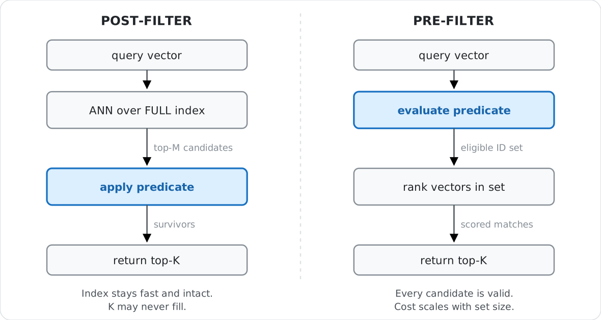
The highlighted box is the only difference that matters, and everything downstream follows from it. Each plan has a slice of the workload where it is the right call, and a slice where it falls off a cliff.
The post-filter cliff: silent incompleteness
Post-filtering is what most stacks do by default, because it asks nothing of the index. Fetch M, throw away whatever fails the predicate, return K.
That works beautifully as long as most vectors near the query pass the filter. Then the pass rate drops:
usable results ≈ candidates retrieved × local filter pass rate
               ≈ 100 × 1%
               ≈ 1
You asked for ten results and got one. The engine didn’t do anything wrong. It returned the nearest 100 vectors faithfully. They just happened to belong to the wrong tenant, region, or quarter.
So you over-fetch, because that’s the obvious lever. At a 1% pass rate you need something like 1,000 candidates before you can expect ten matches, and more than that if you want a margin. Completeness is dropping and the work is going up, both at once, and not gently:
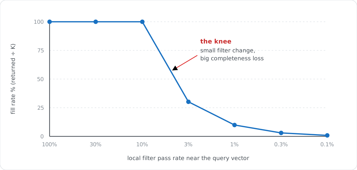
The shape is the thing, not the exact numbers. A user narrowing a date range by one month is enough to walk your query from the flat part down to the floor.
Takeaway. Post-filtering fails quietly. The query returns
200 OKwith two results in it and nothing anywhere says “incomplete”. If you aren’t measuring fill rate, you’ll hear about this from a customer rather than a dashboard.
The pre-filter cliff: the awkward middle
Pre-filtering has cleaner semantics. Work out the eligible set, then score only inside it. If the filter leaves 500 rows, scoring all 500 exactly is both quick and perfectly accurate. Small filtered sets are the easy case, and exact search is the right answer for them.
The pain is in the middle: a set that’s too big to brute-force cheaply, and too sparse for graph traversal to work.
Most ANN indexes are graphs, and traversal leans on neighbours as stepping stones. A vector that fails your filter can still be the only route to one that passes:
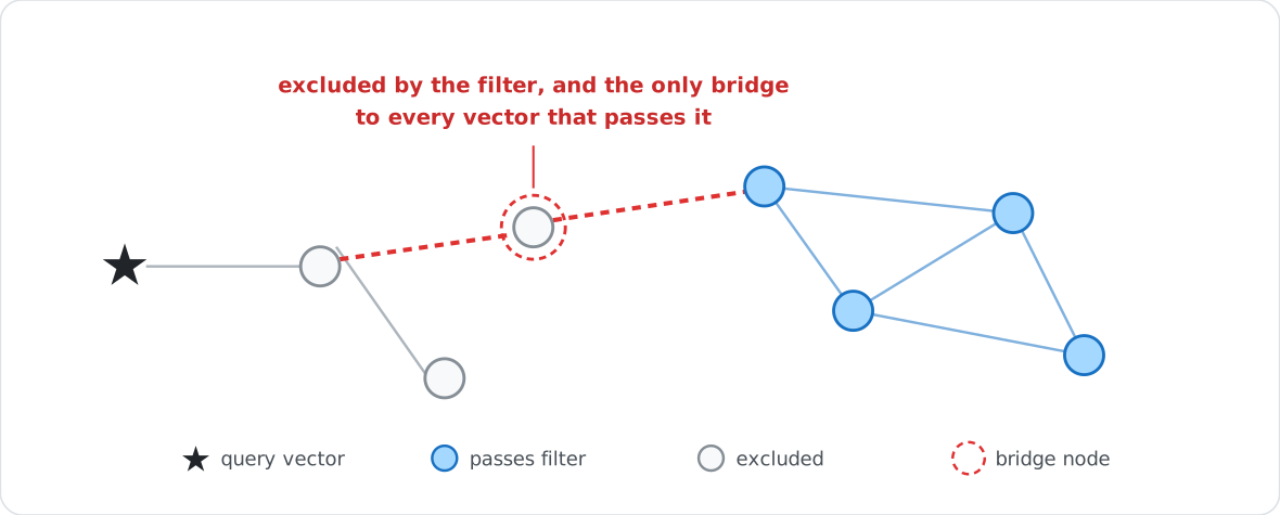
Block that bridge and recall collapses. Let the search walk through it but only collect matches, and you burn visits on nodes you have to discard anyway. Give up and materialise every eligible ID to score directly, and you’re back to a scan whose cost tracks the size of the filtered population.
Takeaway. Pre-filtering swaps a correctness problem for a cost problem. It can’t hand back an invalid result, but it can wreck your p99. In graph indexes it can also lose recall quietly, which looks exactly like a bad embedding model, and that’s usually where the next two weeks go.
The number that actually matters
Global selectivity, as in “this filter matches 10% of the table”, is the number everyone reaches for. It’s also the wrong one. What drives behaviour is the local pass rate in the neighbourhood of the query vector.
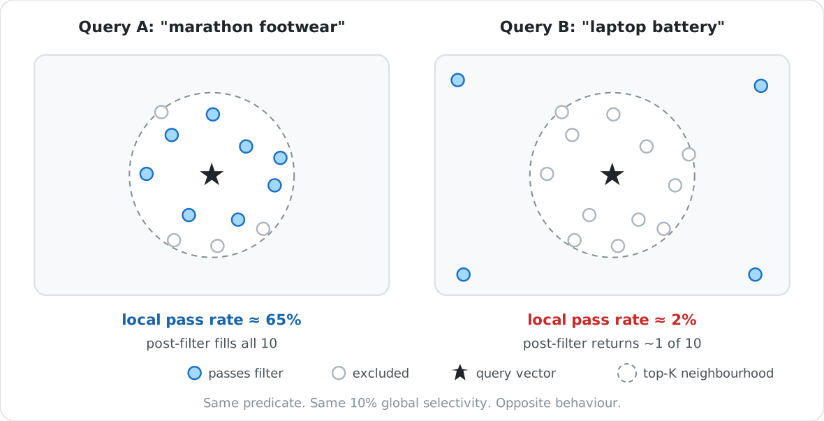
Same predicate. Same 10% global selectivity. Opposite behaviour.
Metadata and embedding distance tend to be correlated, often strongly. A category that’s rare across the whole corpus can form one tight semantic cluster and be trivial to search. A common one can be almost absent from a particular neighbourhood. That’s why a planner working only from row counts will pick the wrong strategy, and why a benchmark built on random predicates tells you close to nothing about production.
Takeaway. Stop quoting global selectivity in design docs. Ask the other question instead: for the filters our users actually send, how many of the top few hundred neighbours survive?
Decide per query, not per system
Treat filtering as a planning decision you make at query time, with a fallback that protects correctness:
| Situation | Plan |
|---|---|
| Eligible set very small | Pre-filter, exact vector scoring |
| High local pass rate | Post-filter with modest over-fetch |
| Selective or embedding-correlated | Filter-aware ANN traversal |
Returned fewer than K | Raise the budget, then fall back to exact |
For the post-filter path, a sane starting budget is:
candidate budget ≈ K ÷ estimated local pass rateTreat it as an estimate, put a ceiling on the over-fetch, and keep the fallback. Where you draw the line between exact and approximate should come from your own dimensions, index, hardware, and latency target. There’s no portable percentage that holds across engines, and anyone who gives you one is guessing.
Filter-aware ANN is the third option, and increasingly the right one. Research systems like Filtered-DiskANN and ACORN push the predicate into traversal instead of applying it before or after, which is what makes the selective-and-correlated case tractable at all. Several commercial engines now ship some version of this. Whether yours does, and whether it covers the predicate shapes you actually use rather than just single-label equality, is worth asking your vendor directly.
Takeaway. “Which filtering strategy did we pick?” isn’t a question you settle once at design time. What you want is a planning rule plus a fallback, so you never silently return an incomplete result.
What to measure
The most common mistake I see is benchmarking an unfiltered index and assuming the numbers carry over. Test the filter combinations your users actually send, and track:
- Fill rate. How often the query returns all
Kresults. This is your cliff detector. - Filtered recall. Against exact search over the eligible set, not against unfiltered search.
- p95 and p99 latency. Averages hide knees by construction.
- Candidates examined per result. This is what the cliff is costing you.
- Pass-rate buckets. 100%, 10%, 1%, 0.1%. Report each one separately, never pooled.
- Correlated vs random predicates. The gap between them is your correlation penalty.
Then add tenant and category skew on top. A plan tuned on your biggest tenant often behaves differently across a long tail of small ones, and that tail is usually most of your customers.
The takeaway
Pre-filtering protects validity, and it can turn search into a scan or break graph navigation. Post-filtering keeps the index fast, and it can quietly hand back incomplete results. Both are correct answers to different workloads, and no single choice survives contact with real user filters.
Which means “does it support metadata filters?” is a weak question to ask a vendor. They all say yes. Ask this instead:
How does the plan change as the eligible set shrinks and the local pass rate falls, and what does the engine do when it can’t fill
K?
Measure those things across the filters your users really send, and the cliff stops being a mystery incident. It turns into a curve you can see, and plan around.
References
- S. Gollapudi et al., “Filtered-DiskANN: Graph Algorithms for Approximate Nearest Neighbor Search with Filters”.
- L. Patel et al., “ACORN: Performant and Predicate-Agnostic Search Over Vector Embeddings and Structured Data”.
- J. Engels et al., “Approximate Nearest Neighbor Search with Window Filters”.